Split Transform Method

In this example we will demonstrate the split transform method for analyzing the imaging performance of a mirror. We begin as usual by importing the relevant classes.

from prysm import Interferogram, Pupil, PSF, sample_files

from matplotlib import pyplot as plt
%matplotlib inline
plt.style.use('bmh')

p = sample_files('dat')  # sample Zygo .dat file, will be downloaded on demand and saved locally
i = Interferogram.from_zygo_dat(p)
i.crop().mask('circle', 40).crop()
i.remove_piston_tiptilt_power()
i.plot2d(clim=100, interpolation=None)  # verify the phase looks OK
plt.grid(False)

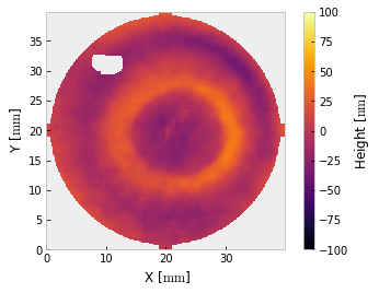
If you are dissatisfied with the masking prowess of prysm, it is recommended to use the software that came with your interferometer. The order of operations from here is very important. Because prysm modifies these classes in-place, we should propagate the PSF before filling the interferogram for PSF analysis.

pu = Pupil.from_interferogram(i)
psf = PSF.from_pupil(pu, efl=200, Q=2)  # F/2
i.fill()

<prysm.interferogram.Interferogram at 0x7f4e5c395f50>

We can then plot,

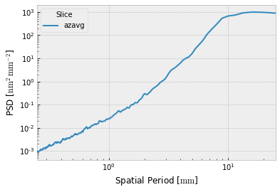
fig, ax = plt.subplots()
i.psd().slices().plot('azavg', fig=fig, ax=ax, invert_x=True, xlim=(25, 0.25), lw=2)
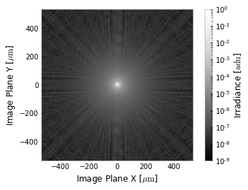
fig, ax = plt.subplots()
# bicubic is highly recommended when the view is small with many pixels
psf.plot2d(xlim=psf.support / 2,
           clim=(1e-9,1e0), log=True,
           interpolation='bicubic',
           fig=fig, ax=ax)
plt.grid(False)